<?xml version="1.0" encoding="utf-8"?><feed xmlns="http://www.w3.org/2005/Atom" ><generator uri="https://jekyllrb.com/" version="3.10.0">Jekyll</generator><link href="https://erykwalczak.github.io/feed.xml" rel="self" type="application/atom+xml" /><link href="https://erykwalczak.github.io/" rel="alternate" type="text/html" /><updated>2026-07-06T21:13:24+01:00</updated><id>https://erykwalczak.github.io/feed.xml</id><title type="html">Eryk Walczak</title><subtitle>Eryk Walczak — Senior Trader at the Bank of England, previously BIS Innovation Hub and BoE Advanced Analytics. Data science, financial markets, and innovation.</subtitle><author><name>Eryk Walczak</name></author><entry><title type="html">Preparing for and passing BCS Foundation Certificate in Business Analysis (v4)</title><link href="https://erykwalczak.github.io/blog/preparing-for-and-passing-bcs-foundation-certificate-in-business-analysis-v4/" rel="alternate" type="text/html" title="Preparing for and passing BCS Foundation Certificate in Business Analysis (v4)" /><published>2023-03-05T13:12:32+00:00</published><updated>2023-03-05T13:12:32+00:00</updated><id>https://erykwalczak.github.io/blog/preparing-for-and-passing-bcs-foundation-certificate-in-business-analysis-v4</id><content type="html" xml:base="https://erykwalczak.github.io/blog/preparing-for-and-passing-bcs-foundation-certificate-in-business-analysis-v4/"><![CDATA[<p>Last week I passed the <a href="https://www.bcs.org/qualifications-and-certifications/certifications-for-professionals/business-analysis/foundation-certificate-in-business-analysis/">BCS Business Analysis Foundation</a> exam. Preparation took me about a week, with a good deal of cramming over one weekend — though I'd already covered a lot of the material on an earlier project management course.</p>
<p>My approach was to:</p>
<ul>
  <li>use the <a href="https://www.bcs.org/media/1944/ba-foundation-syllabus.pdf">syllabus</a> as a starting point;</li>
  <li>make sure I understood the topics it highlights;</li>
  <li>take <a href="/images/blog/2023/03/BCS-v4-Business-Analysis-Syllabus-and-Cheatsheet-Exam-Prep.pdf">notes</a> from the <a href="https://amzn.to/41Otc0U">Business Analysis book</a>; and</li>
  <li>sit several <a href="https://quizlet.com/ie/448050560/business-analysis-sample-paper-2-flash-cards/">mock exams</a>.</li>
</ul>
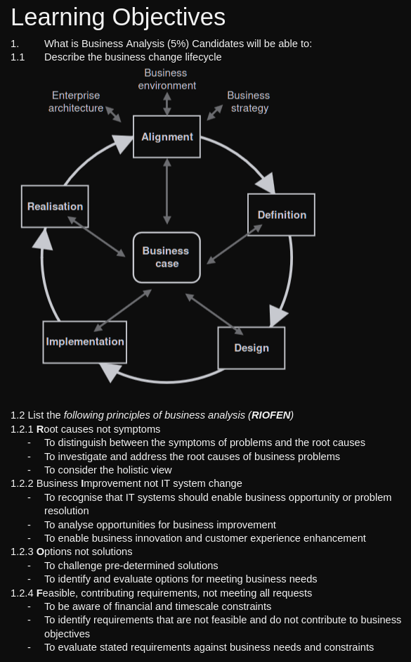
<p>The book can be a little dry on its own, but it's useful for fleshing out the syllabus and practising likely questions. If you're short on time, you can <a href="/images/blog/2023/03/BCS-v4-Business-Analysis-Syllabus-and-Cheatsheet-Exam-Prep.pdf">download my exam notes</a>, which cover the whole syllabus (38 pages, with links to mock exams).</p>
<figure class="wp-block-image size-full is-resized"><a href="/images/blog/2023/03/image.png"><img src="/images/blog/2023/03/image.png" alt="BCS Business Analysis Foundation - Syllabus - Learning Objectives" class="wp-image-782" width="267" height="429" /></a></figure>
<p>It's still worth reading the textbook if you have the time. Here's the edition I used:</p>
<figure class="wp-block-image size-full is-resized"><a href="https://amzn.to/41Otc0U"><img src="/images/blog/2023/03/image-1.png" alt="Business Analysis textbook cover" class="wp-image-783" width="260" height="388" /></a></figure>
<p>Good luck!</p>]]></content><author><name>Eryk Walczak</name></author><category term="Book review" /><category term="Tutorial" /><category term="bcs" /><category term="business-analysis" /><category term="cheatsheet" /><category term="syllabus" /><category term="test-prep" /><summary type="html"><![CDATA[Last week I passed the BCS Business Analysis Foundation exam. Preparation took me about a week, with a good deal of cramming over one weekend — though I'd already covered a lot of the material on an earlier project management course. My approach was to: use the syllabus as a starting point; make sure I understood the topics it highlights; take notes from the Business Analysis book; and sit several mock exams. The book can be a little dry on its own, but it's useful for fleshing out the syllabus and practising likely questions. If you're short on time, you can download my exam notes, which cover the whole syllabus (38 pages, with links to mock exams). It's still worth reading the textbook if you have the time. Here's the edition I used: Good luck!]]></summary></entry><entry><title type="html">PostcodesioR 0.1.1 is on CRAN</title><link href="https://erykwalczak.github.io/blog/postcodesior-0-1-1-is-on-cran/" rel="alternate" type="text/html" title="PostcodesioR 0.1.1 is on CRAN" /><published>2019-08-28T23:40:32+01:00</published><updated>2019-08-28T23:40:32+01:00</updated><id>https://erykwalczak.github.io/blog/postcodesior-0-1-1-is-on-cran</id><content type="html" xml:base="https://erykwalczak.github.io/blog/postcodesior-0-1-1-is-on-cran/"><![CDATA[<h2>Introduction</h2>
<p>The latest stable version of my UK geocoder package has finally made it to <a href="https://cran.r-project.org/web/packages/PostcodesioR/index.html">CRAN</a>. PostcodesioR is a wrapper for <a href="http://postcodes.io/">postcodes.io</a> and it provides multiple functions to work with UK geospatial data.</p>
<p>The package draws exclusively on open data from the Ordnance Survey and the Office for National Statistics, served up as an API by postcodes.io.</p>
<p>PostcodesioR is aimed at data scientists and social scientists working with geocoded UK data. A common task is aggregating data across administrative levels, for example rolling postcode-level data up into counties or regions. The package helps with that, and with plenty of other everyday geospatial jobs.</p>
<h2>Installation</h2>
<p>The package can be installed from CRAN with</p>
<pre class="wp-block-preformatted"><code>install.packages("PostcodesioR")</code></pre>

<p>or from GitHub</p>
<pre class="wp-block-preformatted"><code>devtools::install_github("erykwalczak/PostcodesioR")</code></pre>

<p>Once the package is installed, load it with <code>library(PostcodesioR)</code>.</p>
<h2>Examples</h2>
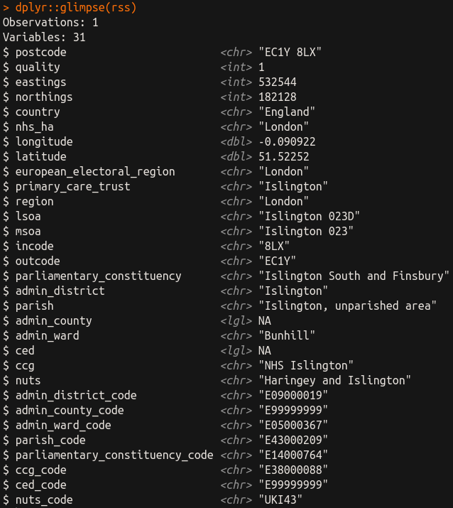
<p>The workhorse of the package is the <code>postcode_lookup()</code> function, which takes a postcode and returns a data frame with the following fields:</p>
<ul><li><code><strong>postcode</strong></code> Postcode. All current ('live') postcodes within the United Kingdom, the Channel Islands and the Isle of Man, received monthly from Royal Mail. 2, 3 or 4-character outward code, single space and 3-character inward code.</li><li><code><strong>quality</strong></code> Positional Quality. Shows the status of the assigned grid reference.</li><li><code><strong>eastings</strong></code> Eastings. The Ordnance Survey postcode grid reference Easting to 1 metre resolution; blank for postcodes in the Channel Islands and the Isle of Man. Grid references for postcodes in Northern Ireland relate to the Irish Grid system.</li><li><code><strong>northings</strong></code> Northings. The Ordnance Survey postcode grid reference Easting to 1 metre resolution; blank for postcodes in the Channel Islands and the Isle of Man. Grid references for postcodes in Northern Ireland relate to the Irish Grid system.</li><li><code><strong>country</strong></code> Country. The country (i.e. one of the four constituent countries of the United Kingdom or the Channel Islands or the Isle of Man) to which each postcode is assigned.</li><li><code><strong>nhs_ha</strong></code> Strategic Health Authority. The health area code for the postcode.</li><li><code><strong>longitude</strong></code> Longitude. The WGS84 longitude given the Postcode's national grid reference.</li><li><code><strong>latitude</strong></code> Latitude. The WGS84 latitude given the Postcode's national grid reference.</li><li><code><strong>european_electoral_region</strong></code> European Electoral Region (EER). The European Electoral Region code for each postcode.</li><li><code><strong>primary_care_trust</strong></code> Primary Care Trust (PCT). The code for the Primary Care areas in England, LHBs in Wales, CHPs in Scotland, LCG in Northern Ireland and PHD in the Isle of Man; there are no equivalent areas in the Channel Islands. Care Trust/ Care Trust Plus (CT) / local health board (LHB) / community health partnership (CHP) / local commissioning group (LCG) / primary healthcare directorate (PHD).</li><li><code><strong>region</strong></code> Region (formerly GOR). The Region code for each postcode. The nine GORs were abolished on 1 April 2011 and are now known as 'Regions'. They were the primary statistical subdivisions of England and also the areas in which the Government Offices for the Regions fulfilled their role. Each GOR covered a number of local authorities.</li><li><code><strong>lsoa</strong></code> 2011 Census lower layer super output area (LSOA). The 2011 Census lower layer SOA code for England and Wales, SOA code for Northern Ireland and data zone code for Scotland.</li><li><code><strong>msoa</strong></code> 2011 Census middle layer super output area (MSOA). The 2011 Census middle layer SOA (MSOA) code for England and Wales and intermediate zone for Scotland.</li><li><code><strong>incode</strong></code> Incode. 3-character inward code that is following the space in the full postcode.</li><li><code><strong>outcode</strong></code> Outcode. 2, 3 or 4-character outward code. The part of postcode before the space.</li><li><code><strong>parliamentary_constituency</strong></code> Westminster Parliamentary Constituency. The Westminster Parliamentary Constituency code for each postcode.</li><li><code><strong>admin_district</strong></code> District. The current district/unitary authority to which the postcode has been assigned.</li><li><code><strong>parish</strong></code> Parish (England)/ community (Wales). The smallest type of administrative area in England is the parish (also known as 'civil parish'); the equivalent units in Wales are communities.</li><li><code><strong>admin_county</strong></code> County. The current county to which the postcode has been assigned.</li><li><code><strong>admin_ward</strong></code> Ward. The current administrative/electoral area to which the postcode has been assigned.</li><li><code><strong>ccg</strong></code> Clinical Commissioning Group. Clinical commissioning groups (CCGs) are NHS organisations set up by the Health and Social Care Act 2012 to organise the delivery of NHS services in England.</li><li><code><strong>nuts</strong></code> Nomenclature of Units for Territorial Statistics (NUTS) / Local Administrative Units (LAU) areas. The LAU2 code for each postcode. NUTS is a hierarchical classification of spatial units that provides a breakdown of the European Union's territory for producing regional statistics which are comparable across the Union. The NUTS area classification in the United Kingdom comprises current national administrative and electoral areas, except in Scotland where some NUTS areas comprise whole and/or part Local Enterprise Regions. NUTS levels 1-3 are frozen for a minimum of three years and NUTS levels 4 and 5 are now Local Administrative Units (LAU) levels 1 and 2 respectively.</li><li><code><strong>_code</strong></code> Returns an ID or Code associated with the postcode. Typically these are a 9 character code known as an ONS Code or GSS Code. This is currently only available for districts, parishes, counties, CCGs, NUTS and wards.</li></ul>
<p>One postcode can be geocoded in the following way</p>
<pre class="wp-block-preformatted"><code>rss &lt;- postcode_lookup("EC1Y8LX")</code></pre>

<figure class="wp-block-image"><img src="/images/blog/2019/08/PostcodesioR_postcode_lookup-1.png" alt="" class="wp-image-708" /></figure>
<p>More than one postcode can be geocoded using <a href="https://purrr.tidyverse.org/">purrr</a></p>
<pre class="wp-block-preformatted"><code>postcodes &lt;- c("EC1Y8LX", "SW1X 7XL")
postcodes_df &lt;- purrr::map_df(postcodes, postcode_lookup)</code></pre>

<p>The remaining functions are demonstrated in the <a href="https://docs.ropensci.org/PostcodesioR/articles/Introduction.html">vignette</a>.</p>
<h2>Documentation and participation</h2>
<p>To read the full documentation of the PostcodesioR package, you can follow <a href="https://docs.ropensci.org/PostcodesioR/">this link</a> to the pkgdown site.</p>
<p>If you want to help with developing the package, report bugs or propose pull requests, you will find the GitHub page <a href="https://github.com/ropensci/PostcodesioR">here</a>.</p>]]></content><author><name>Eryk Walczak</name></author><category term="R package" /><category term="CRAN" /><category term="Geocoding" /><category term="geospatial" /><category term="Map" /><category term="R" /><category term="R-bloggers" /><category term="ropensci" /><category term="UK" /><summary type="html"><![CDATA[Introduction The latest stable version of my UK geocoder package has finally made it to CRAN. PostcodesioR is a wrapper for postcodes.io and it provides multiple functions to work with UK geospatial data. The package draws exclusively on open data from the Ordnance Survey and the Office for National Statistics, served up as an API by postcodes.io. PostcodesioR is aimed at data scientists and social scientists working with geocoded UK data. A common task is aggregating data across administrative levels, for example rolling postcode-level data up into counties or regions. The package helps with that, and with plenty of other everyday geospatial jobs. Installation The package can be installed from CRAN with install.packages("PostcodesioR")]]></summary></entry><entry><title type="html">Extracting pitch track from audio files into a data frame</title><link href="https://erykwalczak.github.io/blog/extracting-pitch-track-from-audio-files-into-a-data-frame/" rel="alternate" type="text/html" title="Extracting pitch track from audio files into a data frame" /><published>2019-02-16T01:15:23+00:00</published><updated>2019-02-16T01:15:23+00:00</updated><id>https://erykwalczak.github.io/blog/extracting-pitch-track-from-audio-files-into-a-data-frame</id><content type="html" xml:base="https://erykwalczak.github.io/blog/extracting-pitch-track-from-audio-files-into-a-data-frame/"><![CDATA[<p>My task was to extract pitch values from a long list of audio files. <a href="/blog/automatic-pitch-extraction-from-speech-recordings/">Previously</a> I'd used Praat and R for this, but looping in R was rather slow, so I went looking for another approach. I developed the following on Linux (Ubuntu).</p>
<p>First, I tried <a href="https://aubio.org/manual/latest/cli.html#aubiopitch">aubio</a> (a CLI-only Python tool) to extract pitch from WAV files. aubio has fewer options than Praat and returned some odd values on its default settings, so I didn't pursue it — though it is easy to use, nicely simple, and Python-native. To extract pitch with aubio:</p>
<pre class="wp-block-code"><code>sudo apt install aubio-tools
aubiopitch -i P17_trim_short_10.000-11.150.wav</code></pre>

<p>In the end I stuck with Praat, the workhorse of phonetics, which can also be driven from the command line.</p>
<p>Praat records every command you run, which is a great starting point for a script. There's more on Praat scripting <a href="http://praatscripting.lingphon.net/introduction.html">here</a>. My solution is below:</p>
<figure class="wp-block-embed"><div class="wp-block-embed__wrapper">
<script src="https://gist.github.com/erykwalczak/53acd493d29ef894bd0870b55d9874ce.js"> </script>
</div></figure>
<p>This script extracts a .<em>pitch</em> file from every .<em>wav</em> file in the working directory and saves them to a subfolder. Praat scripts can be called from the command line:</p>
<pre class="wp-block-code"><code>praat --run extract_pitch_script.praat</code></pre>

<p>This extracts pitch tracks from every .wav file in the directory, using Praat's <a href="http://www.fon.hum.uva.nl/praat/manual/Intro_4__Pitch_analysis.html">default</a> settings, and produces one .<em>pitch</em> file per .<em>wav</em> file. Those files list all the candidates and aren't in a tidy format, so they need transforming. I could probably have done this in Praat scripting too, but I ran out of patience and switched to R, which produces the output I wanted with far less effort.</p>
<p>R can be called from the command line with <a href="https://cran.r-project.org/web/packages/littler/vignettes/littler-examples.html">littler</a>; the shebang on the first line is what makes that possible. The script below turns the .<em>pitch</em> files into clean .<em>csv</em> files.</p>
<figure class="wp-block-embed"><div class="wp-block-embed__wrapper">
<script src="https://gist.github.com/erykwalczak/ff2aabea6ecbde47bde095a1c89f05a6.js"> </script>
</div></figure>
<p>To invoke the R script, run in the command line:</p>
<pre class="wp-block-code"><code>r praat_pitch_analysis_CLI.R untitled_script.pitch</code></pre>

<p>This creates a .<em>csv</em> file holding the best candidate pitch above a given confidence threshold. The pitch extraction algorithm Praat uses was developed by Boersma (<a href="http://www.fon.hum.uva.nl/paul/papers/Proceedings_1993.pdf">1993</a>).</p>]]></content><author><name>Eryk Walczak</name></author><category term="Signal processing" /><category term="Tutorial" /><category term="aubio" /><category term="audio" /><category term="CLI" /><category term="F0" /><category term="pitch" /><category term="Praat" /><category term="Python" /><category term="R" /><category term="speech" /><category term="tone" /><summary type="html"><![CDATA[My task was to extract pitch values from a long list of audio files. Previously I'd used Praat and R for this, but looping in R was rather slow, so I went looking for another approach. I developed the following on Linux (Ubuntu). First, I tried aubio (a CLI-only Python tool) to extract pitch from WAV files. aubio has fewer options than Praat and returned some odd values on its default settings, so I didn't pursue it — though it is easy to use, nicely simple, and Python-native. To extract pitch with aubio: sudo apt install aubio-tools aubiopitch -i P17_trim_short_10.000-11.150.wav]]></summary></entry><entry><title type="html">Automatic splitting of audio files on silence in Python</title><link href="https://erykwalczak.github.io/blog/automatic-splitting-audio-files-silence-python/" rel="alternate" type="text/html" title="Automatic splitting of audio files on silence in Python" /><published>2019-02-11T00:30:39+00:00</published><updated>2019-02-11T00:30:39+00:00</updated><id>https://erykwalczak.github.io/blog/automatic-splitting-audio-files-silence-python</id><content type="html" xml:base="https://erykwalczak.github.io/blog/automatic-splitting-audio-files-silence-python/"><![CDATA[<p>In my previous <a href="/blog/automatic-pitch-extraction-from-speech-recordings/">post</a>, I described how to split audio files into chunks in R. This time I wanted to use Python to prepare long audio files (.<em>mp3</em>) for further analysis. The typical use case is splitting a long recording that contains many words, utterances, or syllables that then need analysing separately — a recorded word list, say.</p>
<p>I ran this on Linux (Ubuntu 16.04). It should be much the same on macOS, but Windows would need a fair few tweaks.</p>
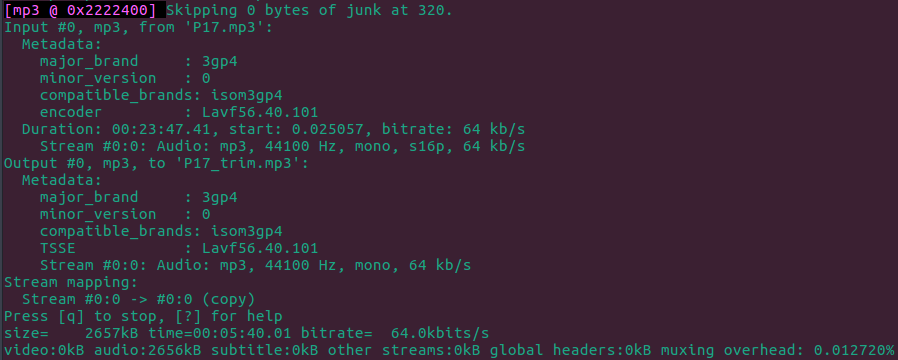
<p>The first step was to convert the original .<em>m4a</em> files into .<em>mp3</em> and extract the segment I cared about. I used <a href="https://ffmpeg.org/">ffmpeg</a> for both. You can skip this if your files are already clean.</p>
<pre class="wp-block-code"><code>ffmpeg -i P17.m4a P17.mp3﻿
ffmpeg -i P17.mp3 -ss 00:17:50 -to 00:23:30 -c copy P17_trim.mp3</code></pre>

<p>The second command copied the original .<em>mp3</em> and extracted the segment between 17:50 and 23:30 — the part of my file that contained speech.</p>
<figure class="wp-block-image"><img src="/images/blog/2019/02/ffmpeg_crop_segment_mp3.png" alt="" class="wp-image-647" /><figcaption>ffmpeg output</figcaption></figure>
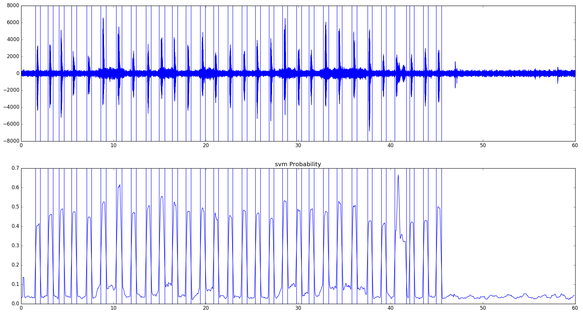
<p>My continuous audio file contained repeated utterances of the same syllable. The code below splits it into segments, using a <a href="https://en.wikipedia.org/wiki/Support_vector_machine">support vector machine</a> (SVM) to detect silence:</p>
<p>Install <a href="https://github.com/tyiannak/pyAudioAnalysis">pyAudioAnalysis</a> and run this on the command line:</p>
<pre class="wp-block-code"><code>python pyAudioAnalysis/pyAudioAnalysis/audioAnalysis.py silenceRemoval -i P17_trim_short.mp3 --smoothing 1.0 --weight 0.3﻿</code></pre>

<figure class="wp-block-image"><a href="/images/blog/2019/02/pyAudioAnalysis_silenceRemoval.png"><img src="/images/blog/2019/02/pyAudioAnalysis_silenceRemoval-1024x555.png" alt="pyAudioAnalysis detect silence in audio files" class="wp-image-651" /></a><figcaption>The top row shows the waveform of the audio signal (amplitude on the y-axis, time on the x-axis). The bottom row shows the probability of non-silence; the vertical lines are the markers used to split the file.</figcaption></figure>
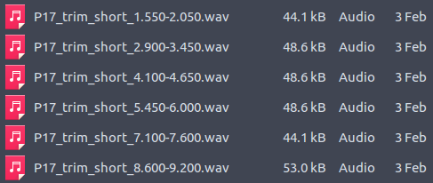
<p>The result is a list of sliced wav files. The names contain timings of the boundaries.</p>
<figure class="wp-block-image"><img src="/images/blog/2019/02/pyAudioAnalysis_split_wav_files.png" alt="" class="wp-image-653" /><figcaption>pyAudioAnalysis silenceRemoval output example.</figcaption></figure>
<p>All files in a given directory can be split using the following script:</p>
<figure class="wp-block-embed"><div class="wp-block-embed__wrapper">
<script src="https://gist.github.com/erykwalczak/5b28ae422b8a5cef91f91967c657bf9c.js"> </script>
</div></figure>
<p>Make sure to point the script at the directory where <em>audioAnalysis.py</em> lives. Adjusting the <em>smoothing</em> and <em>weight</em> parameters changes the results, so tune them to suit the type of recording. By default the script pops up a window showing the suggested split, which is handy for keeping an eye on data quality. Run it from the command line with:</p>
<pre class="wp-block-code"><code>python split_continuous_audio.py</code></pre>]]></content><author><name>Eryk Walczak</name></author><category term="Signal processing" /><category term="Tutorial" /><category term="audio" /><category term="chunk" /><category term="CLI" /><category term="Python" /><category term="segmentation" /><category term="slicing" /><category term="speech" /><summary type="html"><![CDATA[In my previous post, I described how to split audio files into chunks in R. This time I wanted to use Python to prepare long audio files (.mp3) for further analysis. The typical use case is splitting a long recording that contains many words, utterances, or syllables that then need analysing separately — a recorded word list, say. I ran this on Linux (Ubuntu 16.04). It should be much the same on macOS, but Windows would need a fair few tweaks. The first step was to convert the original .m4a files into .mp3 and extract the segment I cared about. I used ffmpeg for both. You can skip this if your files are already clean. ffmpeg -i P17.m4a P17.mp3﻿ ffmpeg -i P17.mp3 -ss 00:17:50 -to 00:23:30 -c copy P17_trim.mp3]]></summary></entry><entry><title type="html">Book Review - Sound Analysis and Synthesis with R</title><link href="https://erykwalczak.github.io/blog/book-review-sound-analysis-and-synthesis-with-r/" rel="alternate" type="text/html" title="Book Review - Sound Analysis and Synthesis with R" /><published>2018-11-03T17:38:00+00:00</published><updated>2018-11-03T17:38:00+00:00</updated><id>https://erykwalczak.github.io/blog/book-review-sound-analysis-and-synthesis-with-r</id><content type="html" xml:base="https://erykwalczak.github.io/blog/book-review-sound-analysis-and-synthesis-with-r/"><![CDATA[<p>R might not be the most obvious choice for analysing audio data, but a growing number of packages now make it possible to analyse and synthesise sound. One of them is seewave, and <a href="https://scholar.google.com/citations?user=wH4U0ygAAAAJ&amp;hl=en">Jérôme Sueur</a>, one of its authors, has written a book on working with audio data in R. It’s called <a href="https://www.springer.com/us/book/9783319776453">Sound Analysis and Synthesis with R</a>, published by Springer in 2018, and I’d highly recommend it to anyone working with audio.</p>

<p><a href="https://www.springer.com/us/book/9783319776453"><img class="aligncenter size-full wp-image-637" src="/images/blog/2018/10/Sound-Analysis-and-Synthesis-with-R-book-cover.png" alt="" width="289" height="439" /></a></p>

<p>The book opens with a general explanation of sound, then introduces R to readers with no prior experience. Across its 17 chapters, the author works through the basic audio analyses you can do in R, explaining the underlying concepts with both mathematical equations and R code. There’s some material on sound synthesis too, though it’s a minor theme next to the space given to analysis. The <a href="https://link.springer.com/chapter/10.1007%2F978-3-319-77647-7_1">supplementary materials</a> include the sound samples used throughout.</p>

<p>As I said, the book’s main focus is analysing sound, mostly in scientific settings. Researchers and data scientists typically want to load, visualise, play, and quantify a particular sound, and the book covers these basics with code examples that are easy to follow and richly illustrated with R-generated plots. You can preview it <a href="https://books.google.co.uk/books?id=zfVeDwAAQBAJ&amp;lpg=PR1&amp;pg=PR13#v=onepage&amp;q&amp;f=false">here</a>.</p>

<p>If you ever need to paste, delete, repeat, or reverse audio files in R, you’ll find recipes for all of them here. The book also has twenty <em>DIY Boxes</em>, which show alternative ways to use the functions already covered and demonstrate new tasks, ranging from loading and plotting audio files to frequency and amplitude analysis.</p>

<p>Although the author created his own package, the book also shows how to use a wide range of other audio-specific R packages, such as <a href="https://cran.r-project.org/web/packages/tuneR/index.html">tuneR</a> and <a href="https://cran.r-project.org/web/packages/warbleR/index.html">warbleR</a>.</p>

<p>My only wish is that this book had come out sooner — it would have saved me a lot of pain doing audio analyses.</p>

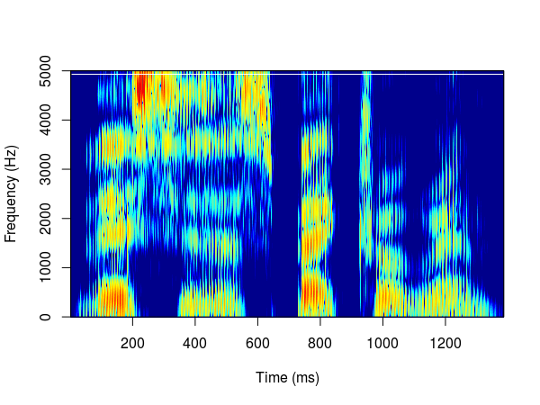
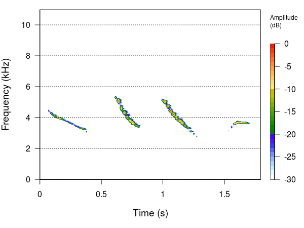
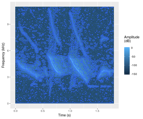
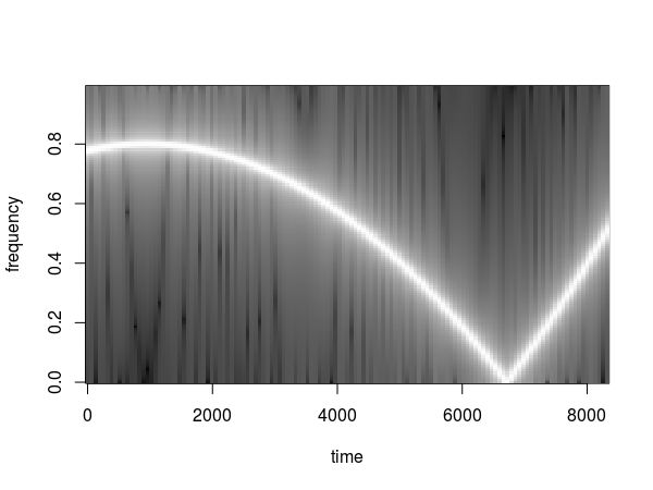
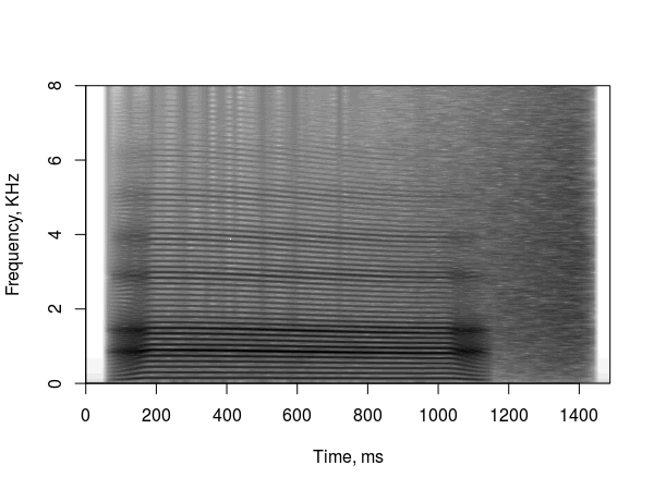
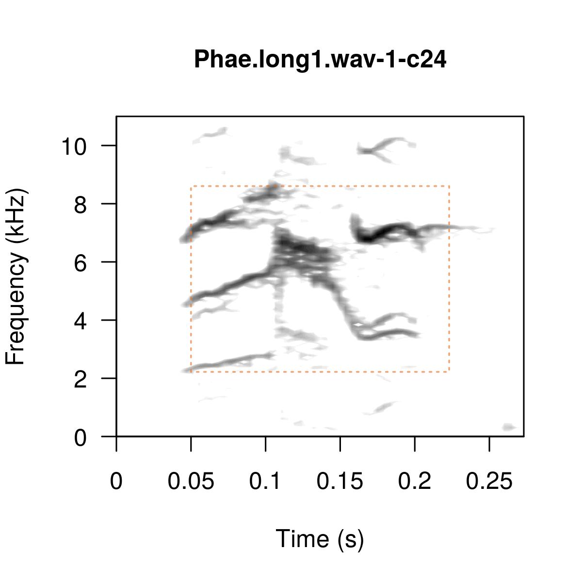
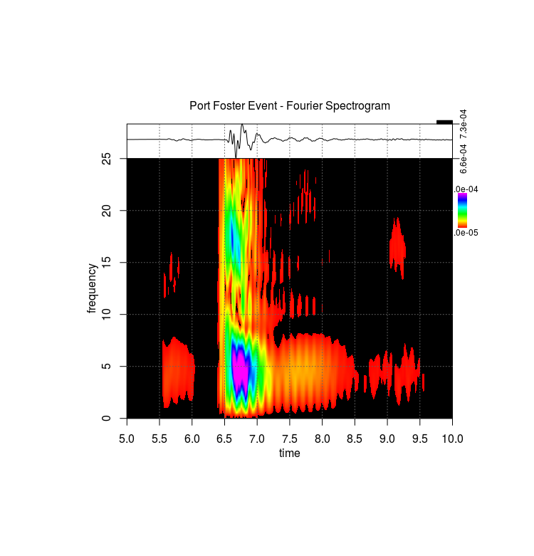
<p>Final verdict: <strong>5/5</strong></p>]]></content><author><name>Eryk Walczak</name></author><category term="Book review" /><category term="audio" /><category term="R" /><category term="R-bloggers" /><category term="sound" /><category term="speech" /><category term="synthesis" /><summary type="html"><![CDATA[R might not be the most obvious choice for analysing audio data, but a growing number of packages now make it possible to analyse and synthesise sound. One of them is seewave, and Jérôme Sueur, one of its authors, has written a book on working with audio data in R. It’s called Sound Analysis and Synthesis with R, published by Springer in 2018, and I’d highly recommend it to anyone working with audio.]]></summary></entry><entry><title type="html">Spectrograms in R - a gallery</title><link href="https://erykwalczak.github.io/blog/spectrograms-in-r-a-gallery/" rel="alternate" type="text/html" title="Spectrograms in R - a gallery" /><published>2018-09-01T14:19:34+01:00</published><updated>2018-09-01T14:19:34+01:00</updated><id>https://erykwalczak.github.io/blog/spectrograms-in-r-a-gallery</id><content type="html" xml:base="https://erykwalczak.github.io/blog/spectrograms-in-r-a-gallery/"><![CDATA[<p>Creating a <a href="https://en.wikipedia.org/wiki/Spectrogram">spectrogram</a> is a basic step in almost any analysis of audio signals — it shows how the frequencies in a sound change over time. Happily, R has a good few packages for the job, and here I’ll run through the ones I like to use. This post isn’t an introduction to spectrograms themselves; if you want the theory, try other resources, such as these <a href="https://www.phon.ucl.ac.uk/courses/spsci/acoustics/week1-10.pdf">lecture notes</a> from UCL.</p>

<p>The examples below come mostly from the official documentation and are kept as simple as possible. Most of the functions let you customise the plots further.</p>

<p><a href="https://cran.r-project.org/web/packages/phonTools/index.html">phonTools</a>
<script src="https://gist.github.com/erykwalczak/bff84ae4295f396116a95029c6fdf8fa.js"> </script>
<a href="/images/blog/2018/09/phonTools_spectrogram_R.png"><img src="/images/blog/2018/09/phonTools_spectrogram_R.png" alt="" width="600" height="450" class="aligncenter size-full wp-image-622" /></a></p>

<p><a href="https://cran.r-project.org/web/packages/seewave/index.html">seewave</a>
<script src="https://gist.github.com/erykwalczak/c419edc571d02f1ed7c3712046fd72b8.js"> </script>
<a href="/images/blog/2018/09/seewave_spectrogram_R.png"><img src="/images/blog/2018/09/seewave_spectrogram_R.png" alt="" width="600" height="450" class="aligncenter size-full wp-image-624" /></a></p>

<p><a href="https://cran.r-project.org/web/packages/seewave/index.html">seewave</a> and <a href="https://cran.r-project.org/web/packages/ggplot2/index.html">ggplot2</a>
<script src="https://gist.github.com/erykwalczak/67757c0bf8ae936a7da422aa36764366.js"> </script>
<a href="/images/blog/2018/09/seewave_ggplot2_spectrogram_R.png"><img src="/images/blog/2018/09/seewave_ggplot2_spectrogram_R.png" alt="" width="600" height="450" class="aligncenter size-full wp-image-623" /></a></p>

<p><a href="https://cran.r-project.org/web/packages/signal/index.html">signal</a>
<script src="https://gist.github.com/erykwalczak/85bddaa15f6a5fd780c1d49c2d64e47e.js"> </script>
<a href="/images/blog/2018/09/signal_spectrogram_R.png"><img src="/images/blog/2018/09/signal_spectrogram_R.png" alt="" width="600" height="450" class="aligncenter size-full wp-image-625" /></a></p>

<p><a href="https://cran.r-project.org/web/packages/soundgen/index.html">soundgen</a>
<script src="https://gist.github.com/erykwalczak/e114baf74913108feb3c8906de0e1918.js"> </script>
<a href="/images/blog/2018/09/soundgen_spectrogram_R.png"><img src="/images/blog/2018/09/soundgen_spectrogram_R.png" alt="" width="600" height="450" class="aligncenter size-full wp-image-626" /></a></p>

<p><a href="https://cran.r-project.org/web/packages/warbleR/index.html">warbleR</a>
<script src="https://gist.github.com/erykwalczak/b3cddfe92fe74662f6658d71d5d665ad.js"> </script>
<a href="/images/blog/2018/09/Phae.long1_.wav-1.jpeg"><img src="/images/blog/2018/09/Phae.long1_.wav-1-1024x1024.jpeg" alt="" width="640" height="640" class="aligncenter size-large wp-image-621" /></a></p>

<p><a href="https://cran.r-project.org/web/packages/hht/index.html">hht</a>
<script src="https://gist.github.com/erykwalczak/6fa4a88eef6e35c08d9a674ae6efe488.js"> </script>
<a href="/images/blog/2018/09/hht_spectrogram_R.png"><img src="/images/blog/2018/09/hht_spectrogram_R.png" alt="" width="750" height="781" class="aligncenter size-full wp-image-620" /></a></p>

<p>Creating a spectrogram from the scratch is not so difficult, as shown by Hansen Johnson in <a href="https://hansenjohnson.org/post/spectrograms-in-r/">this blog post</a>. Another <a href="https://github.com/usagi5886/dsp/blob/master/Spectrogram().r">solution</a> was provided by Aaron Albin.
<script src="https://gist.github.com/erykwalczak/89247b920d5536dbf3f36ab7c2b6c2af.js"> </script>
<a href="/images/blog/2018/09/Spectrogram_R.png"><img src="/images/blog/2018/09/Spectrogram_R.png" alt="" width="600" height="500" class="aligncenter size-full wp-image-627" /></a></p>

<p><a href="http://www.fon.hum.uva.nl/praat/">Praat</a> is a workhorse of audio analysis. It is a standalone software, but there is also an R controller called <a href="http://aaronalbin.com/praatr/index.html">PraatR</a>, that allows calling Praat functions from R. It is not the easiest tool to use so I will just mention it here for reference.</p>

<p>I am pretty sure that there are more packages that allow creating spectrograms but I had to stop somewhere. Feel free to leave comments about other examples.</p>]]></content><author><name>Eryk Walczak</name></author><category term="Data visualisation" /><category term="Signal processing" /><category term="Tutorial" /><category term="audio" /><category term="R" /><category term="R-bloggers" /><category term="spectrogram" /><category term="speech" /><summary type="html"><![CDATA[Creating a spectrogram is a basic step in almost any analysis of audio signals — it shows how the frequencies in a sound change over time. Happily, R has a good few packages for the job, and here I’ll run through the ones I like to use. This post isn’t an introduction to spectrograms themselves; if you want the theory, try other resources, such as these lecture notes from UCL.]]></summary></entry><entry><title type="html">Removing triggers from Hitachi ETG-4000 fNIRS recordings</title><link href="https://erykwalczak.github.io/blog/removing-triggers-from-hitachi-etg-4000-fnirs-recordings/" rel="alternate" type="text/html" title="Removing triggers from Hitachi ETG-4000 fNIRS recordings" /><published>2018-04-12T21:06:19+01:00</published><updated>2018-04-12T21:06:19+01:00</updated><id>https://erykwalczak.github.io/blog/removing-triggers-from-hitachi-etg-4000-fnirs-recordings</id><content type="html" xml:base="https://erykwalczak.github.io/blog/removing-triggers-from-hitachi-etg-4000-fnirs-recordings/"><![CDATA[<p>HOMER2 expects a particular .nirs format that can’t contain consecutive triggers (also called <em>Marks</em> in Hitachi files). The <a href="https://www.nitrc.org/projects/hitachi2nirs">hitachi2nirs</a> MATLAB script does strip the markers, but I wanted to recreate the whole process myself and be sure I was doing it correctly. Answering Yes to <em>Do you want to remove the marker at the end of each stimulus? y/n</em> runs the following code:
<script src="https://gist.github.com/erykwalczak/01bdb34377e02a4405d4da9f8099279c.js"> </script>
To remove the triggers in R, follow the steps below.</p>

<p>Start by loading the packages and files:
<script src="https://gist.github.com/erykwalczak/b19ba983d3b4d87322d28a937f1af854.js"> </script>
This produces a table showing the structure:</p>

<div class="language-plaintext highlighter-rouge"><div class="highlight"><pre class="highlight"><code>## 'data.frame':    2500 obs. of  50 variables:
##  $ Probe1      : int  1 2 3 4 5 6 7 8 9 10 ...
##  $ CH1.703.6.  : num  0.1865 0.0182 -0.4738 -0.1521 -0.3078 ...
##  $ CH1.829.0.  : num  0.412 0.547 0.534 0.314 0.106 ...
##  $ CH2.703.9.  : num  0.739 0.764 0.746 0.751 0.762 ...
##  $ CH2.829.3.  : num  1.01 1.01 1.03 1.03 1.03 ...
##  $ CH3.703.9.  : num  1.57 1.58 1.59 1.59 1.6 ...
##  $ CH3.829.3.  : num  1.64 1.65 1.65 1.66 1.67 ...
##  $ CH4.703.9.  : num  1.48 1.45 1.55 1.51 1.47 ...
##  $ CH4.828.8.  : num  1.63 1.64 1.66 1.66 1.68 ...
##  $ CH5.703.6.  : num  -1.226 -1.743 -0.546 -0.556 -0.75 ...
##  $ CH5.829.0.  : num  0.00397 -0.23102 -1.11099 -0.64056 -1.01425 ...
##  $ CH6.703.1.  : num  -0.247 -0.335 -0.371 -0.667 -1.064 ...
##  $ CH6.828.8.  : num  0.987 0.892 0.892 0.933 0.796 ...
##  $ CH7.703.9.  : num  1.03 1.3 1.11 1.02 1.44 ...
##  $ CH7.829.3.  : num  1.2 1.22 1.21 1.23 1.23 ...
##  $ CH8.702.9.  : num  2 2.01 2.03 2.04 2.04 ...
##  $ CH8.829.0.  : num  1.79 1.81 1.81 1.83 1.85 ...
##  $ CH9.703.9.  : num  2.07 2.02 2.12 2.12 2.01 ...
##  $ CH9.828.8.  : num  1.82 1.82 1.82 1.84 1.85 ...
##  $ CH10.703.1. : num  -0.492 -0.135 -0.598 -0.598 -0.328 ...
##  $ CH10.828.8. : num  0.672 0.61 0.823 0.724 0.724 ...
##  $ CH11.703.1. : num  -1.042 -0.255 -1.773 -1.419 -0.449 ...
##  $ CH11.828.8. : num  1.071 1.052 0.804 1.107 1.047 ...
##  $ CH12.702.9. : num  0.684 0.771 0.704 0.512 0.905 ...
##  $ CH12.829.0. : num  1.02 1.01 1.03 1.08 1.07 ...
##  $ CH13.702.9. : num  2.03 2.03 2.05 2.05 2.05 ...
##  $ CH13.829.0. : num  1.76 1.78 1.79 1.79 1.81 ...
##  $ CH14.703.6. : num  -1.719 -1.196 -0.359 -0.883 -1.99 ...
##  $ CH14.829.0. : num  -0.0832 0.0209 -0.1123 -0.2014 -0.2011 ...
##  $ CH15.703.1. : num  1.97 1.89 1.82 1.98 2.09 ...
##  $ CH15.828.8. : num  1.81 1.78 1.8 1.81 1.84 ...
##  $ CH16.703.4. : num  0.0209 -0.4283 -0.0848 -0.278 0.4996 ...
##  $ CH16.829.0. : num  1.36 1.26 1.38 1.23 1.27 ...
##  $ CH17.702.9. : num  2.35 2.35 2.36 2.37 2.38 ...
##  $ CH17.829.0. : num  2.08 2.09 2.11 2.12 2.13 ...
##  $ CH18.703.6. : num  2.1 2.1 2.09 2.1 2.1 ...
##  $ CH18.828.5. : num  2.14 2.14 2.14 2.15 2.15 ...
##  $ CH19.703.6. : num  -1.104 -1.134 -0.658 -0.886 -0.336 ...
##  $ CH19.829.0. : num  -0.1239 0.09369 0.05463 0.01617 -0.00427 ...
##  $ CH20.703.4. : num  1.65 1.55 1.28 1.35 1.56 ...
##  $ CH20.829.0. : num  1.77 1.75 1.8 1.81 1.8 ...
##  $ CH21.703.4. : num  1.41 1.43 1.31 1.42 1.46 ...
##  $ CH21.829.0. : num  1.76 1.77 1.76 1.77 1.79 ...
##  $ CH22.703.6. : num  2.11 2.29 2.18 2.24 2.21 ...
##  $ CH22.828.5. : num  2.17 2.17 2.18 2.17 2.2 ...
##  $ Mark        : int  0 0 0 0 0 0 0 0 0 0 ...
##  $ Time        : num  0 0.1 0.2 0.3 0.4 0.5 0.6 0.7 0.8 0.9 ...
##  $ BodyMovement: int  0 0 0 0 0 0 0 0 0 0 ...
##  $ RemovalMark : int  0 0 0 0 0 0 0 0 0 0 ...
##  $ PreScan     : int  1 1 1 1 1 1 1 1 1 1 ...
</code></pre></div></div>

<p>It also gives a table of the triggers:</p>

<div class="language-plaintext highlighter-rouge"><div class="highlight"><pre class="highlight"><code>## .
##  1  2  9 10 
## 73 10  4  2
</code></pre></div></div>

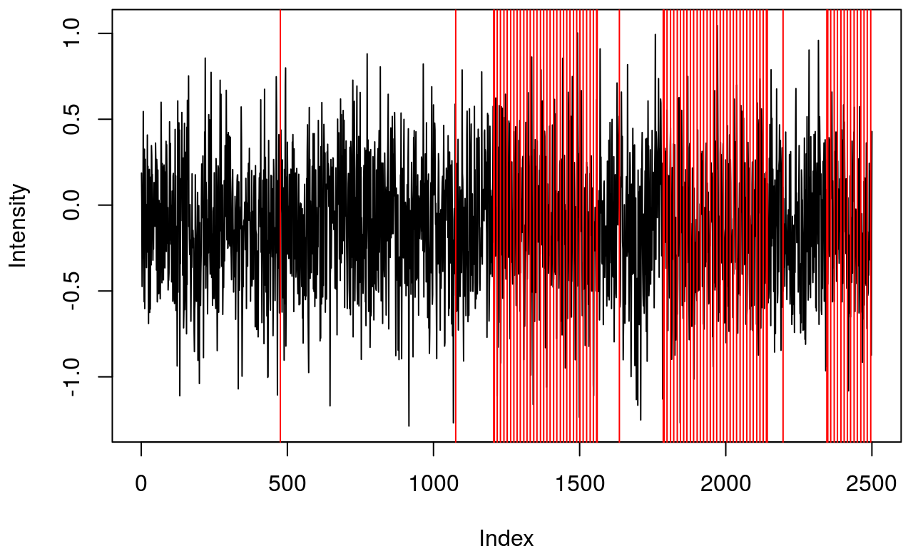
<p>and a plot of the raw data for one channel (rather noisy) with all the triggers marked.
<a href="/images/blog/2018/04/hitachi2nirs_plot1.png"><img src="/images/blog/2018/04/hitachi2nirs_plot1-1024x624.png" alt="" width="640" height="390" class="aligncenter size-large wp-image-601" /></a></p>

<p>There are several triggers here (all shown in red). I only want to keep trigger ‘2’, which marks the start of a block, so the first step is to strip out everything else.
<script src="https://gist.github.com/erykwalczak/5d22d19d811f630c3a3d70ee7961ff20.js"> </script>
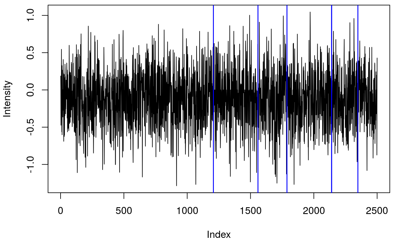
That leaves fewer events:
<a href="/images/blog/2018/04/hitachi2nirs_plot2.png"><img src="/images/blog/2018/04/hitachi2nirs_plot2-1024x623.png" alt="" width="640" height="389" class="aligncenter size-large wp-image-602" /></a></p>

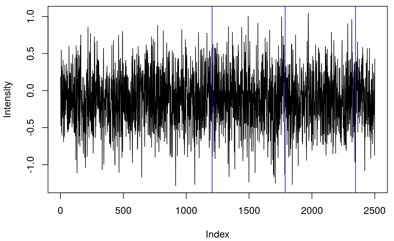
<p>It turned out there were two ‘2’ triggers side by side. This is because the ETG-4000 doesn’t allow odd triggers next to each other — 212 is invalid, but 22111122 is fine. I wrote a function (soon to be folded into the <a href="https://github.com/erykwalczak/fnirsr">fnirsr</a> package) to handle this.
<script src="https://gist.github.com/erykwalczak/9a360692db54e9f1bdacbe29e7dd3743.js"> </script>
The result, showing only the first block’s events, is below:
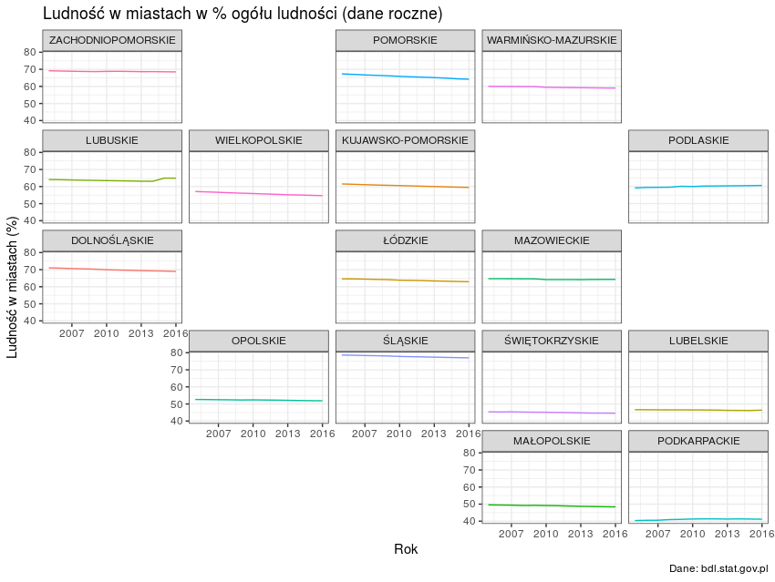
<a href="/images/blog/2018/04/hitachi2nirs_plot3.png"><img src="/images/blog/2018/04/hitachi2nirs_plot3-1024x625.png" alt="" width="640" height="391" class="aligncenter size-large wp-image-603" /></a></p>]]></content><author><name>Eryk Walczak</name></author><category term="Neuroscience" /><category term="Signal processing" /><category term="Tutorial" /><category term="fNIRS" /><category term="Time series" /><summary type="html"><![CDATA[HOMER2 expects a particular .nirs format that can’t contain consecutive triggers (also called Marks in Hitachi files). The hitachi2nirs MATLAB script does strip the markers, but I wanted to recreate the whole process myself and be sure I was doing it correctly. Answering Yes to Do you want to remove the marker at the end of each stimulus? y/n runs the following code: To remove the triggers in R, follow the steps below.]]></summary></entry><entry><title type="html">Geofacet Polski - wykresy w miejscu województw</title><link href="https://erykwalczak.github.io/blog/geofacet-polski-wykresy-w-miejscu-wojewodztw/" rel="alternate" type="text/html" title="Geofacet Polski - wykresy w miejscu województw" /><published>2018-03-25T21:40:23+01:00</published><updated>2018-03-25T21:40:23+01:00</updated><id>https://erykwalczak.github.io/blog/geofacet-polski-wykresy-w-miejscu-wojewodztw</id><content type="html" xml:base="https://erykwalczak.github.io/blog/geofacet-polski-wykresy-w-miejscu-wojewodztw/"><![CDATA[<p>Niedawno odnalazłem ciekawy pakiet <a href="https://hafen.github.io/geofacet/">geofacet</a>, który umożliwia rozmieszczenie wykresów zgodnie z ich pozycją na mapie. Główna funkcja <em>facet_geo()</em> zastępuje <em>facet_wrap()</em> z ggplot2. Polska mapa jeszcze nie jest dostępna w standardowym pakiecie geofacet, ale mam nadzieję, że już wkrótce tam się znajdzie, bo dodałem ją na <a href="https://github.com/hafen/geofacet/issues/95">GitHubie</a>.</p>

<p>Stworzyłem siatkę z koordynatami poszczególnych województw. Wykresy z pakietem geofacet mogą wyglądać tak:</p>

<p><a href="/images/blog/2018/03/geofacet_polska_poland_wojewodztwa.png"><img class="aligncenter wp-image-691 size-full" src="/images/blog/2018/03/geofacet_polska_poland_wojewodztwa.png" alt="geofacet_polska_poland_wojewodztwa" width="850" height="639" /></a>
Rozmieszczenie województw nie jest idealne, ale pakiet geofacet umożliwia użycie własnych ustawień.</p>

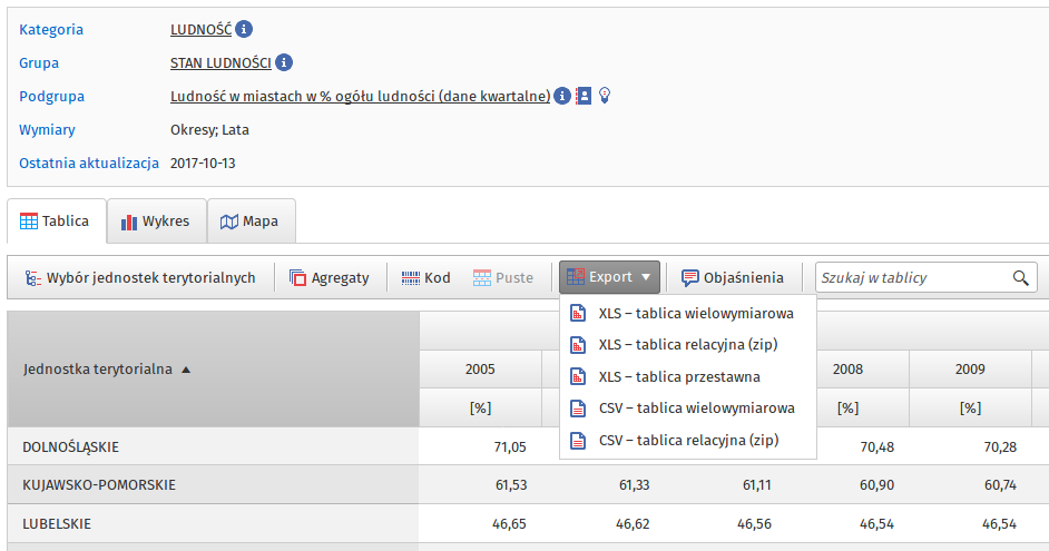
<p>Dane pochodzą z <a href="https://bdl.stat.gov.pl/BDL/start">Banku Danych Lokalnych</a> (<em>XLS - tablica przestawna</em>)</p>

<p><a href="/images/blog/2018/03/bank_danych_lokalnych_ludnosc_w_miastach.png"><img class="aligncenter size-medium wp-image-583" src="/images/blog/2018/03/bank_danych_lokalnych_ludnosc_w_miastach-300x158.png" alt="" width="300" height="158" /></a></p>

<p>Kod do stworzenia wykresów:
<script src="https://gist.github.com/erykwalczak/5973fe9f33bb18db5797d63c2e952cda.js"> </script></p>]]></content><author><name>Eryk Walczak</name></author><category term="Data visualisation" /><category term="Tutorial" /><category term="Map" /><category term="Mapa Polski" /><category term="R" /><summary type="html"><![CDATA[Niedawno odnalazłem ciekawy pakiet geofacet, który umożliwia rozmieszczenie wykresów zgodnie z ich pozycją na mapie. Główna funkcja facet_geo() zastępuje facet_wrap() z ggplot2. Polska mapa jeszcze nie jest dostępna w standardowym pakiecie geofacet, ale mam nadzieję, że już wkrótce tam się znajdzie, bo dodałem ją na GitHubie.]]></summary></entry><entry><title type="html">Downloading UK property prices from Zoopla in R</title><link href="https://erykwalczak.github.io/blog/downloading-uk-property-prices-from-zoopla-in-r/" rel="alternate" type="text/html" title="Downloading UK property prices from Zoopla in R" /><published>2018-01-07T01:56:56+00:00</published><updated>2018-01-07T01:56:56+00:00</updated><id>https://erykwalczak.github.io/blog/downloading-uk-property-prices-from-zoopla-in-r</id><content type="html" xml:base="https://erykwalczak.github.io/blog/downloading-uk-property-prices-from-zoopla-in-r/"><![CDATA[<p>Zoopla offers limited access to its <a href="https://developer.zoopla.co.uk/">API</a>, which serves up the latest property prices and area indices. I wrote an R package for querying it — see the GitHub <a href="https://github.com/erykwalczak/zooplaR">documentation</a> or <a href="https://erykwalczak.github.io/zooplaR/">zooplaR’s page</a> for the latest.</p>

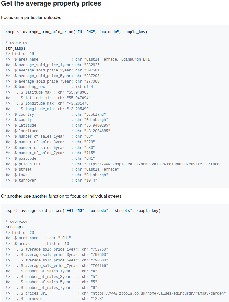
<p><a href="/images/blog/2018/01/zooplaR_UK_average_property_prices_api.png"><img src="/images/blog/2018/01/zooplaR_UK_average_property_prices_api.png" alt="" width="735" height="968" class="aligncenter size-full wp-image-561" /></a></p>

<p>It’s easy to pull prices over the last few months or years for a given postcode, outcode, or area:
<script src="https://gist.github.com/erykwalczak/4a17ab3912191e620f2eecefc0bffc2e.js"> </script>
Given the limited number of queries, it can be worth sanity-checking the results against the property widget Zoopla provides (it redirects to zoopla.co.uk).</p>

<p>The widget has fewer options than the API and isn’t automated, but it’s handy for a quick cross-check.</p>

<div id="zoopla_search"><div class="zoopla_header"><span><a href="https://www.zoopla.co.uk/" rel="nofollow">Property search</a></span></div>

<script type="text/javascript" src="https://www.zoopla.co.uk/widgets/scripts/partner_widgets/search.js?type_rent=1&amp;type_sale=1&amp;type_values=1&amp;type_prices=1"></script>

<div class="zoopla_powered"><span>Powered by Zoopla.co.uk</span></div></div>]]></content><author><name>Eryk Walczak</name></author><category term="R package" /><category term="API" /><category term="proptech" /><category term="R" /><category term="R-bloggers" /><category term="UK house prices" /><category term="Zoopla" /><summary type="html"><![CDATA[Zoopla offers limited access to its API, which serves up the latest property prices and area indices. I wrote an R package for querying it — see the GitHub documentation or zooplaR’s page for the latest.]]></summary></entry><entry><title type="html">Enabling MATLAB in Jupyter notebooks on Linux</title><link href="https://erykwalczak.github.io/blog/enabling-matlab-in-jupyter-notebooks-on-linux/" rel="alternate" type="text/html" title="Enabling MATLAB in Jupyter notebooks on Linux" /><published>2017-11-06T23:42:38+00:00</published><updated>2017-11-06T23:42:38+00:00</updated><id>https://erykwalczak.github.io/blog/enabling-matlab-in-jupyter-notebooks-on-linux</id><content type="html" xml:base="https://erykwalczak.github.io/blog/enabling-matlab-in-jupyter-notebooks-on-linux/"><![CDATA[<h2>Introduction</h2>

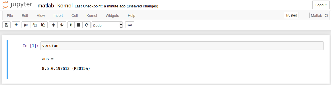
<p>In my previous <a href="/blog/using-matlab-in-jupyter-notebooks-on-windows/">post</a>, I showed how to enable MATLAB in Jupyter notebooks on Windows. Now it’s the turn of GNU/Linux (Ubuntu).</p>

<p><a href="/images/blog/2017/11/matlab_jupyter_kernel_linux.png"><img src="/images/blog/2017/11/matlab_jupyter_kernel_linux.png" alt="" width="1153" height="298" class="aligncenter size-full wp-image-544" /></a></p>

<p>My main headache with enabling the new kernel was having started out with two Anaconda installs and two Python versions (2.7 and 3.5). After a lot of frustration, I wiped both Anacondas and did a clean install of the latest Anaconda with Python 2.7 and 3.5. This tutorial assumes you already have Jupyter and MATLAB installed.</p>

<h2>Using the right environment</h2>

<p>Although the official MATLAB website says the Python-MATLAB engine works with Python 2.7, 3.4, 3.5, and 3.6, I couldn’t get it to install under Python 3.5. If you try, you’ll see this error:</p>

<p><em>OSError: MATLAB Engine for Python supports Python version 2.7, 3.3 and 3.4, but your version of Python is 3.5</em></p>

<p>The error makes it clear you need an older version of Python. I went with 2.7, creating a dedicated environment for it:</p>

<p><code class="language-plaintext highlighter-rouge">conda create -n py27 python=2.7 anaconda</code></p>

<p>The guidelines to managing Python environments are <a href="https://conda.io/docs/user-guide/tasks/manage-python.html">here</a>.</p>

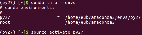
<p>The next step was checking what environments were available:</p>

<p><code class="language-plaintext highlighter-rouge">conda info --envs</code></p>

<p>And activating Python 2.7 (<em>py27</em>):</p>

<p><code class="language-plaintext highlighter-rouge">source activate py27</code></p>

<p><a href="/images/blog/2017/11/matlab_jupyter_linux_conda_envs.png"><img src="/images/blog/2017/11/matlab_jupyter_linux_conda_envs.png" alt="" width="489" height="121" class="aligncenter size-full wp-image-537" /></a></p>

<h2>Install Python-MATLAB engine</h2>

<p>To install the engine that connects the two languages, go to your MATLAB folder, find the Python engine folder, and run <em>setup.py</em>. Here’s how:</p>

<p>Change your working directory to wherever MATLAB lives:
<code class="language-plaintext highlighter-rouge">cd "MATLABROOT/extern/engines/python"</code></p>

<p>If you don’t know where your MATLAB is installed, use:
<code class="language-plaintext highlighter-rouge">locate matlab</code></p>

<p>Then install the engine (it will only work with MATLAB &gt;=2014b):</p>

<p><code class="language-plaintext highlighter-rouge">sudo python setup.py install</code></p>

<p>And the <a href="https://pip.pypa.io/en/stable/reference/pip_install/#cmdoption-u">latest</a> remaining dependencies:</p>

<div class="language-bash highlighter-rouge"><div class="highlight"><pre class="highlight"><code><span class="nb">sudo </span>pip <span class="nb">install</span> <span class="nt">-U</span> metakernel
<span class="nb">sudo </span>pip <span class="nb">install</span> <span class="nt">-U</span> matlab_kernel
<span class="nb">sudo </span>pip <span class="nb">install</span> <span class="nt">-U</span> pymatbridge
</code></pre></div></div>

<p>That should do the job. Now open a new Jupyter notebook:</p>

<p><code class="language-plaintext highlighter-rouge">jupyter notebook</code></p>

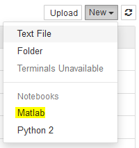
<p>Check whether MATLAB shows up among the available engines (top right corner):</p>

<p><a href="/images/blog/2017/07/Jupyter_MATLAB_choose_language.png"><img src="/images/blog/2017/07/Jupyter_MATLAB_choose_language.png" alt="" width="200" height="213" class="aligncenter size-full wp-image-499" /></a></p>

<p>Then check that the notebook actually runs. When I first tried Python 3.5, MATLAB appeared in the list but the kernel died every time I ran any MATLAB code. Switching to Python 2.7, as described here, fixed it.</p>

<p>If everything’s working, the following notebook should run correctly:
<script src="https://gist.github.com/erykwalczak/a214d1d2fe3c93859e46802714519eea.js"> </script>
Even though I get the MetaKernelApp error below, the notebook still works fine:
<em>[MetaKernelApp] ERROR | No such comm target registered: jupyter.widget.version</em>
<a href="/images/blog/2017/11/MetaKernelApp_error_no_such_comm_matlab.png"><img src="/images/blog/2017/11/MetaKernelApp_error_no_such_comm_matlab.png" alt="" width="978" height="122" class="aligncenter size-full wp-image-541" /></a></p>

<p>To leave the environment used to run the notebook, simply type:</p>

<p><code class="language-plaintext highlighter-rouge">source deactivate</code></p>

<h2>Notes</h2>

<p>I struggled a fair bit to get everything working, and along the way I also installed <a href="https://www.gnu.org/software/octave/">Octave</a> (a free MATLAB equivalent). I’m not sure whether that actually helped with running MATLAB inside Jupyter.</p>

<p>While installing the engine, I ran into several errors. Most were probably down to my OS configuration, and all of them were solved by searching for the error message. One of them was:</p>

<p><em>Error:
[I 00:58:19.847 NotebookApp] KernelRestarter: restarting kernel (3/5)
/home/eub/anaconda3/bin/python: No module named matlab_kernel</em></p>

<p>This was caused by installing the Python engine in the wrong environment (my default Python 3.5). Activating Python 2.7 first, then installing the Python-MATLAB engine from there, sorted it out.</p>

<p>There’s probably an alternative way to enable MATLAB in Jupyter without Anaconda: point the installer explicitly at the Python version that supports the Py-MATLAB engine.</p>

<p>In my case:
<code class="language-plaintext highlighter-rouge">sudo ~/anaconda/pkgs/python-2.7.13-0/bin/python2.7 setup.py install</code></p>

<p>You might also want to install the engine in a non-default location. MATLAB has a <a href="https://uk.mathworks.com/help/matlab/matlab_external/install-matlab-engine-api-for-python-in-nondefault-locations.html">guide</a> for that, which suggests installing Python in your home directory.</p>

<p>There’s also another Jupyter kernel, <a href="https://github.com/imatlab/imatlab">imatlab</a>, which supposedly works with Python 3.5 and MATLAB R2016b onwards, though I haven’t tried it. As long as my current setup keeps working, I’m in no hurry to wrestle with dependencies again.</p>]]></content><author><name>Eryk Walczak</name></author><category term="Tutorial" /><category term="Jupyter" /><category term="Linux" /><category term="MATLAB" /><category term="Python" /><summary type="html"><![CDATA[Introduction]]></summary></entry></feed>